In this posting, I will write down some regex rules that I used in my finance NLP program.
Find surnames and other names from Hong Kong name list
In the Hong Kong name list, the pattern is that the surnames will be all capital words and
other name words will start with capital character and followed by lower-case characters.
Two exampes are D'AQUINO Thomas Paul, DOWSLEY James William D'Altera and E Meng
find_surname=re.compile(r'\b[A-Z]+\'?[A-Z]+\b|^[A-Z]{1}\b')find_othername=re.compile(r'\b[A-Z]{1}\'[A-Z]{1}[a-z]+\b|\b[A-Z]{1}[a-z]+\b|\b [A-Z]{1}-?\b')fullname="D'AQUINO Thomas Paul"find_surname.findall(fullname)find_othername.findall(fullname)
Issues
Find surname in LIE-A-CHEONG Tai Chong David
When I add this pattern to previous regex, I found One problem.
find_surname=re.compile(r'\b[A-Z]+\'?[A-Z]+\b|^[A-Z]{1}\b|\b-[A-Z]{1}-\b')find_surname.findall("LIE-A-CHEONG Tai Chong David")
I installed elasticsearch and related tools on Mac. Firstly you can refer to this website; however there are
still some tricks we need to pay attention.
1. Check if your java is up-to-date.
2. Download and extract Elasticsearch in the directory you want:
curl -L -O https://artifacts.elastic.co/downloads/elasticsearch/elasticsearch-5.2.2.tar.gz
tar -xvf elasticsearch-5.2.2.tar.gz
3. Download and extract Kibana (do not download from start page):
wget https://artifacts.elastic.co/downloads/kibana/kibana-5.2.2-darwin-x86_64.tar.gz
tar -xzf kibana-5.2.2-darwin-x86_64.tar.gz
4. Install X-Pack (for security and authentication) in Elasticsearch install dir:
bin/elasticsearch-plugin install x-pack
5. Install X-Pack in Kibana install dir:
bin/kibana-plugin install x-pack
6. Run Elasticsearch in the default port 9200:
# Under the dir elasticsearch-5.2.2
./bin/elasticsearch -Ecluster.name=my_cluster_name -Enode.name=my_node_name
7. Run Kibana in the default port 5601:
# Under the dir kibana-5.2.2-darwin-x86_64
.bin/kibana
Remarks:
The default username of Elasticsearch for xpack is elastic and password is changeme
The default username of Kibana for xpack is elastic and password is changeme
Command "python setup.py egg_info" failed with error code 1 in /private/var/folders/4v/r8x7ssn916792z84sf7chx740000gn/T/pip-build-m6rki5l0/xgboost/
Then I try the other option in the xgboost documents,
which is to clone the XGBoost github repo and then install:
git clone --recursive https://github.com/dmlc/xgboost
cd xgboost
cp make/config.mk ./config.mk
make -j4
Install system-widely, which requires root permission
cd python-package
sudo python setup.py install
You will however need Python distutils module for this to work. It is often part of the core python package or
it can be installed using your package manager, e.g. in Debian use
sudo apt-get install python-setuptools
If you recompiled xgboost, then you need to reinstall it again to make the new library take effect
Note: you may need to brew tap homebrew/versions and install gcc --without-multilib1 if you did not install gcc-5 or gcc-6 before.
In this part, I will introduce some self-defined functions to choose parameters for classifiers. These functions form one
pipeline to work from feature adjustment (transform categorical variables to dummy variables), stratified sampling, choosing best parameters
combination to print out accuarcy for both training set and testing set.
stratified - stratified index from sklearn.cross_validation.StratifiedKFold
Main Function
defdo_classify(clf,indf,featurenames,targetname,target1val,parameters=None,mask=None,random_state=30,reuse_split=None,stratified=None,dummies=False,score_func=None,n_folds=4,n_jobs=1):y=(indf[targetname].values==target1val)*1ifdummies:X=indf[featurenames]X_train=X.iloc[stratified[0],:]stratified_train=StratifiedKFold(X_train.contbr_st,n_folds=n_folds,random_state=random_state)X=pd.get_dummies(X,prefix='',prefix_sep='').valueselse:X=indf[featurenames].valuesifstratified!=None:stratified=list(stratified)print('using stratified sampling')Xtrain,ytrain=X[stratified[0]],y[stratified[0]]Xtest,ytest=X[stratified[1]],y[stratified[1]]ifmask!=None:print("using mask")Xtrain,Xtest,ytrain,ytest=X[mask],X[~mask],y[mask],y[~mask]ifparameters!=None:ifstratified!=None:clf=cv_optimize(clf,parameters,Xtrain,ytrain,stratified=stratified_train,n_jobs=n_jobs,n_folds=n_folds,score_func=score_func)else:clf=cv_optimize(clf,parameters,Xtrain,ytrain,n_jobs=n_jobs,n_folds=n_folds,score_func=score_func)clf=clf.fit(Xtrain,ytrain)training_accuracy=clf.score(Xtrain,ytrain)test_accuracy=clf.score(Xtest,ytest)print("############# based on standard predict ################")print("Accuracy on training data: %0.2f"%(training_accuracy))print("Accuracy on test data: %0.2f"%(test_accuracy))print(confusion_matrix(ytest,clf.predict(Xtest)))print("########################################################")returnclf,Xtrain,ytrain,Xtest,ytest
Important arguments
indf - Input dataframe
featurenames - vector of names of predictors
targetname - name of column you want to predict (e.g. 0 or 1, ‘M’ or ‘F’,
‘yes’ or ‘no’)
target1val - particular value you want to have as a 1 in the target
mask - boolean vector indicating test set (~mask is training set)
(we’ll use this to test different classifiers on the same
test-train splits)
stratified - list that stores stratified index, normally we can get this from
list(StratifiedKFold(, n_folds=5))[0]. If it is defined, then inside cv_optimize will also apply stratified sampling
dummies - If True, the categorical features will be transformed as dummy variables
score_func - we’ve used the accuracy as a way of scoring algorithms but
this can be more general later on
n_folds - Number of folds for cross validation ()
n_jobs - used for parallelization stratified and mask cannot be simultaneously applied
Remarks
stratified in this model is for stratifying samples based on one specific feature not on the target. It deals with the problem with highly imbalanced categorical feature.
If your target is highly imbalanced, there is one option that you can use is to set class_weight = 'balanced' inside the sklearn classifiers.
One Example
Here is one example from one of my project to predict party preference in 2016 US predencial election based on the donation data set. When I did the feature engineering, there is one tricky issue I need to tackle. After I ruled out all missing data, the numbers of donators for states are really different. For example California has about 60,000 donators, whereas Nevada only has 10 donators. However we still do not want to loss any states when we split data into training set and test set. In this case, the best choice should be stratified sampling strategies.
gbm=xgb.XGBClassifier()skf=list(StratifiedKFold(df_clean.contbr_st,n_folds=5,random_state=30))[0]#Stratifed sampling first, then make variable dummies.featurenames=['contbr_st','employer_categorized','salary','MedianPrice','Gender','is_Retired','is_Unemployed_NotRetired','is_Self_Employed']targetname='party'param={"max_depth":[7,9,11],"n_estimators":[300,400,500],'learning_rate':[0.05,0.08,0.1]}gbm_fitted,Xtrain,ytrain,Xtest,ytest=do_classify(gbm,df_clean,featurenames,targetname,1,stratified=skf,parameters=param,dummies=True,n_jobs=4,n_folds=4)
Self-Defined Classification Functions in Python (Part 1)
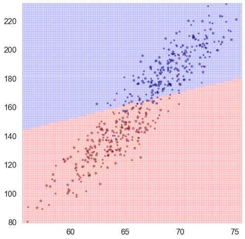
Binary Classification results based on two features
cmap_light=ListedColormap(['#FFAAAA','#AAFFAA','#AAAAFF'])cmap_bold=ListedColormap(['#FF0000','#00FF00','#0000FF'])defclassify_plot(ax,Xtr,Xte,ytr,yte,clf,mesh=True,colorscale=cmap_light,cdiscrete=cmap_bold,alpha=0.1,psize=10):h=.02X=np.concatenate((Xtr,Xte))x_min,x_max=X[:,0].min()-.5,X[:,0].max()+.5y_min,y_max=X[:,1].min()-.5,X[:,1].max()+.5xx,yy=np.meshgrid(np.linspace(x_min,x_max,100),np.linspace(y_min,y_max,100))Z=clf.predict(np.c_[xx.ravel(),yy.ravel()])ZZ=Z.reshape(xx.shape)ifmesh:plt.pcolormesh(xx,yy,ZZ,cmap=colorscale,alpha=alpha,axes=ax)else:showtr=ytrshowte=yteax.scatter(Xtr.iloc[:,0],Xtr.iloc[:,1],c=showtr-1,cmap=cdiscrete,s=psize,alpha=alpha,edgecolor="k")# and testing pointsax.scatter(Xte.iloc[:,0],Xte.iloc[:,1],c=showte-1,cmap=cdiscrete,alpha=alpha,marker="*",s=psize+30)ax.set_xlim(xx.min(),xx.max())ax.set_ylim(yy.min(),yy.max())returnax,xx,yy
Parameters
ax: figure information
Xtr: pandas.DataFrame
Training set of features where features are in the columns
Xte: DataFrame
Testing set of features where features are in the columns
ytr: DataFrame
Training set of target
yte: DataFrame
Testing set of target
clf: fitted classifier
mesh: plot mesh or not. If False, then it only plots predicted values.
colorscale: specify the Colormap for mesh plot
Colormap is the base classes to convert numbers to color to the RGBA color.
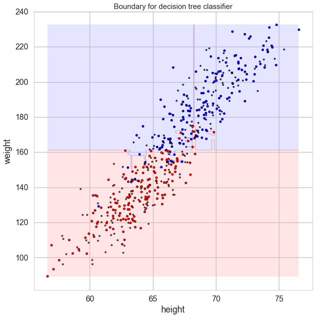
defplot_tree(ax,Xtr,Xte,ytr,yte,clf,plot_train=True,plot_test=True,lab=['Feature 1','Feature 2'],mesh=True,colorscale=cmap_light,cdiscrete=cmap_bold,alpha=0.3,psize=10):# Create a meshgrid as our test dataplt.figure(figsize=(15,10))plot_step=0.05xmin,xmax=Xtr[:,0].min(),Xtr[:,0].max()ymin,ymax=Xtr[:,1].min(),Xtr[:,1].max()xx,yy=np.meshgrid(np.arange(xmin,xmax,plot_step),np.arange(ymin,ymax,plot_step))# Re-cast every coordinate in the meshgrid as a 2D pointXplot=np.c_[xx.ravel(),yy.ravel()]# Predict the classZ=clf.predict(Xplot)# Re-shape the resultsZ=Z.reshape(xx.shape)cs=ax.contourf(xx,yy,Z,cmap=cmap_light,alpha=0.3)# Overlay training samplesif(plot_train==True):ax.scatter(Xtr[:,0],Xtr[:,1],c=ytr-1,cmap=cmap_bold,alpha=alpha,edgecolor="k")# and testing pointsif(plot_test==True):ax.scatter(Xte[:,0],Xte[:,1],c=yte-1,cmap=cmap_bold,alpha=alpha,marker="*")ax.set_xlabel(lab[0])ax.set_ylabel(lab[1])ax.set_title("Boundary for decision tree classifier",fontsize=15)
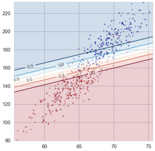
Colormaps is very useful when we try to convert numbers into colors.
If the colormaps have a listed values like ListedColormap(['#FFAAAA', '#AAFFAA', '#AAAAFF']), it means to map one number into one of these three colors. For example if \(X = [x_1, … , x_n]\) has values from 0 to 1, then [0, 0.33] indicates color #FFAAAA, (0.33, 0.66] indicates color #AAFFAA and (0.66, 1] indicates color AAAAFF.
If the colormaps is continuous like plt.cm.RdBu, then the numbers should map to that range. The following is one example:
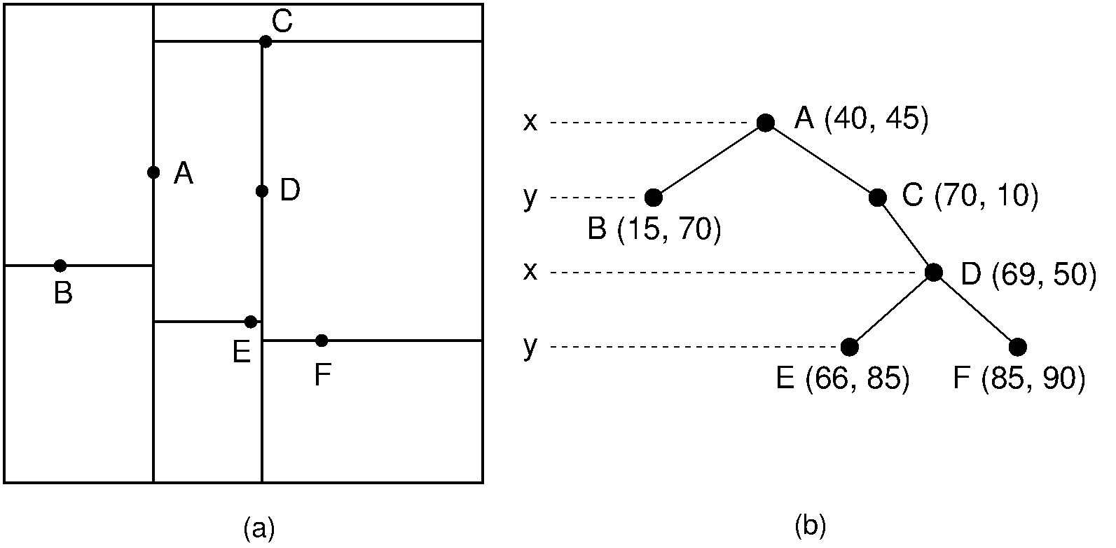
In some cases we may be not interested in the question “is X in this container,” but rather “what value in the container is X most similar to?”
At a high level, a kd-tree is a generalization of a binary search tree that stores points in k-dimensional
space.
This is quoted from this nice introduction,
and you can find more detailed interpretation in it. Here I just excerpt some contents from it.
When we just consider the balanced K-D tree, we always use median value to be split boundaries.
Nearest-Neighbor
The first target should be in the smallest cell and we randomly choose one point in that cell, then we can construct a candidate hy- persphere centered at the test point and running through the guess point. The nearest neighbor to the test point must lie inside this hypersphere.
If this hypersphere is fully to one side of a splitting hyperplane, then all points on the other side of the splitting hyperplane cannot be contained in the sphere and thus cannot be the nearest neighbor.
To determine whether the candidate hypersphere crosses a splitting hyperplane that com- pares coordinate i, we check whether \(|b_i – a_i|<r\).
If this hypersphere crosses some boundaries, we need to go back to the parent node (may go up to multiple upleavls). Then get a point to compute the distance and compare it with the previous distance.
This algorithm can be shown to run in O(log n) time on a balanced kd-tree with n data points provided that those points are randomly distributed. In the worst case, though, the entire tree might have to be searched. However, in low-dimensional spaces, such as the Cartesian plane or three-di- mensional space, this is rarely the case.
k-Nearest Neighbor Searches
We will apply K-D tree with a bounded priority queue (or BPQ for short) to tackle this problem. A bounded priority queue is similar to a regular priority queue, except that there is a fixed upper bound on the number of elements that can be stored in the BPQ. When- ever a new element is added to the queue, if the queue is at capacity, the element with the highest priority value is ejected from the queue.
A generator function is defined like a normal function, but whenever it needs to generate a value, it does so with the yield
keyword rather than return. If the body of a def contains yield, the function automatically becomes a generator function
(even if it also contains a return statement). There’s nothing else we need to do to create one.
Just remember that a generator is a special type of iterator.
In Python, “functions” with these capabilities are called generators, and they’re incredibly useful. generators
(and the yield statement) were initially introduced to give programmers a more straightforward way to write code responsible
for producing a series of values. Previously, creating something like a random number generator required a class or module that
both generated values and kept track of state between calls. With the introduction of generators, this became much simpler.
To better understand the problem generators solve, let’s take a look at an example. Throughout the example, keep in
mind the core problem being solved: generating a series of values.
Outside of Python, all but the simplest generators would be referred to as coroutines.
Stop criteria
If a generator function calls return
If the generator is exhausted by calling next(). After that if we call next() again it will result in an error.
The issue with this implementation is that each function calls two functions and that become exponetial. Think of fib(20). It will call fib(18) and fib(19). fib(19) will call fib(18) and fib(17). So fib(18) gets called 2 times, fib(17) 3 times, etc. And the count goes up exponetially. The same code as above with a counter. fib(20) causes the function to be called over 13K times. Try fib(40)… the code wouldn’t even complete.
100000 loops, best of 3: 2.24 µs per loop
10000 loops, best of 3: 26.3 µs per loop
100000 loops, best of 3: 3.31 µs per loop
So the basic fuction is the best, generator function comes next and recursive function is the worst.
This fibonacci is not a good problem for generator function. I will provide another fancier example. This example is shameless stolen from this blog.
importrandomdefget_data():"""Return 3 random integers between 0 and 9"""returnrandom.sample(range(10),3)defconsume():"""Displays a running average across lists of integers sent to it"""running_sum=0data_items_seen=0whileTrue:data=yielddata_items_seen+=len(data)running_sum+=sum(data)print('The running average is {}'.format(running_sum/float(data_items_seen)))defproduce(consumer):"""Produces a set of values and forwards them to the pre-defined consumer
function"""whileTrue:data=get_data()print('Produced {}'.format(data))consumer.send(data)yieldif__name__=='__main__':consumer=consume()consumer.send(None)producer=produce(consumer)for_inrange(10):print('Producing...')next(producer)
Tips
generators are used to generate a series of values
yield is like the return of generator functions
The only other thing yield does is save the “state” of a generator function
A generator is just a special type of iterator
Like iterators, we can get the next value from a generator using next()
It is common to use while True: inside generator function.
Today in the Metis bootcamp we learnt SQL. I read one book Learning SQL some months ago, but I still need more practice on it. So I take some notes here to remind myself its basic syntax. This practice based on this website.
After one day intense work on setting up Ipython on AWS, I think it worth writing the whole process down. There are too many details that need to care about. Most of the contents here are shameless stolen from Andrew Blevins.
Contents Table
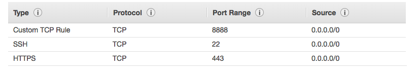
Add the inbound port when setup the instance
Add user and security issue (not necessary)
Download Anaconda and software updates
Setting up Jupyter Notebook
Release Jupyter Notebook from terminal
Add the inbound port when setup the instance
When setup the instance (I used ubuntu instance), we need to add more ports when setup security group:
Adding User and Security
Open AWS server on your local terminal
ssh -i .ssh/aws_key.pem ubuntu@11.11.11.11
Remarks
aws_key.pem is the downloaded password key from aws when we create the instance.
11.11.11.11 is the AWS instance public IP.
This is a public account so it is not safe.
Add new user
ubuntu@ip-172-31-60-68:/home$ sudo adduser jason
Note: pick a password (save it in an easy-to-find place !! ); enter through all the other questions (name fields, etc.)
Delete user
$ sudo userdel -r olduser
User privileges
Make yourself special by granting yourself root privileges: type sudo visudo. This will open up nano (a text editor) to edit the sudoers file. Find the line that says root ALL=(ALL:ALL) ALL. Give yourself a line beneath that which says [username] ALL=(ALL:ALL) ALL.
User privilege specification
root     ALL=(ALL:ALL) ALL
jason  ALL=(ALL:ALL) ALL
Save file in nano editor: Ctrl-o then Enter when asked for the file name. Exit file from nano editor: Ctrl-x
Setting up User Account
Now you have a user account, but you can’t just log in with a password. Passwords aren’t secure enough.
Copy your github public key (from your local machine) ~/.ssh/id_rsa.pub to your remote machine to the authorized keys file. Your github public key may have different name. You need to know your password for this SSH key. Please notice that this password may be not the same one you use to login your github account. If you cannot remember this, you need to reset github public SSH:
Jason@news-MacBook-Pro:~/.ssh$ ssh-keygen -t rsa
Remarks:
After this command you need to rename the public key file or use the default id_rsa.
You will set your password again.
Create the authorized_keys file
On your remote machine (AWS):
create the directory
then copy key from local machine (all characters inside id_rsa.pub) to remote machine.
sudo mkdir -p /home/my_cool_username/.ssh/
sudo vi /home/my_cool_username/.ssh/authorized_keys
When you paste the key please be careful that you may miss the first character ‘s’.
My example:
1)  get output from your (local machine) public key file like this:
jason$ pwd
/Users/jason/.ssh
jason$ cat id_rsa.pub

2) Copy everything (Command c)

3) On your AWS machine:
after you run:
$ sudo nano /home/jason/.ssh/authorized_keys

To paste in the current window:  Command v
then hit
ctrl o (to save)
enter
ctrl x (to exit)
Change login name
Open a new terminal on your local machine under the root directory. Then create a file .ssh/config, in which .ssh is the folder where you put your password key id_rsa.
$vim`.ssh/config`#Then inside config file paste the following lines:
Host machine_name_goes_here
Hostname 123.234.123.234
User my_cool_username
My exsample:
Host aws_ipython
     HostName 54.172.80.98
     User jason
Remarks
Host is the AWS instance name.
HostName is the public IP of the AWS instance
user is the new user name you just created
Now you can log in to your remote machine with ssh machine_name_goes_here.
Send a file from your local machine to your remote machine
$ scp cool_file.png machine_name_goes_here:~
Type exit on your remote machine and open a shell on your local machine:
$ ssh -i .ssh/id_rsa machine_name_goes_here
If you do not change the default user name, you can use the following commands:
scp -i <location of aws key> melville-moby_dick.txt ubuntu@11.11.11.11:~/data/
Remarks:
Please be careful about .ssh/id_rsa, it is not .ssh/id_rsa.pub!!
You need to enter your github password for SSH.
Next time you only need to type ssh machine_name_goes_here to login.
Download Anaconda and software updates
After we use that new user name to login AWS, we need to update python and install Jupyter Notebook. The easest way is to download Anaconda.
jason@ip-172-31-60-68:~$ mkdir .jupyter
jason@ip-172-31-60-68:~$ cd ~/.jupyter/
jason@ip-172-31-60-68:~$ vi jupyter_notebook_config.py
Then you need to copy the following codes into the second line in this file (under # Configuration file for jupyter-notebook.).
c = get_config()# Kernel config
c.IPKernelApp.pylab ='inline'# if you want plotting support always in your notebook# Notebook config
c.NotebookApp.certfile ='/home/my_cool_username/.certs/mycert.pem'#location of your certificate file
c.NotebookApp.ip ='*'
c.NotebookApp.open_browser = False #so that the ipython notebook does not opens up a browser by default
c.NotebookApp.password ='sha1:68c136a5b064...'#the encrypted password we generated in ipython# Set the port to match the port we opened in the security group
c.NotebookApp.port = 8888
Remarks:
This is for Python 3+.
Be careful about c.NotebookApp.certfile line. You need to enter your own path.
Then let’s run it!
$ cd ~
$ mkdir Notebooks
$ cd Notebooks
$ jupyter notebook
After this you need to open your browser and type 11.11.11.11:8888. 11.11.11.11 is your AWS instance public IP.
Release Jupyter Notebook from terminal
Sometimes we may shut down the terminal by mistakes, then all the runnning notebooks will be affected. We can use the following way to avoid this situation
$ nohup jupyter notebook
Output:
nohup: ignoring input and appending output to ‘nohup.out’
Now you cannot do anything in this terminal. Now you can close this terminal.
Kill this Jupyter Notebook
Open a new terminal and login your remote AWS machine.
$ cd Notebooks #this folder is where you run your Jupyter Notebook last time$ lsof nuohup.out
If your program is still running, you can see something like this:
COMMAND    PID  USER   FD   TYPE DEVICE SIZE/OFF   NODE NAME
jupyter-n 3034 jason    1w   REG  202,1      838 269167 nohup.out
jupyter-n 3034 jason    2w   REG  202,1      838 269167 nohup.out
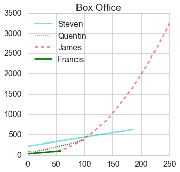
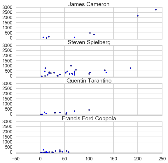
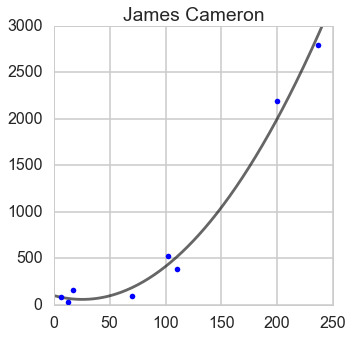
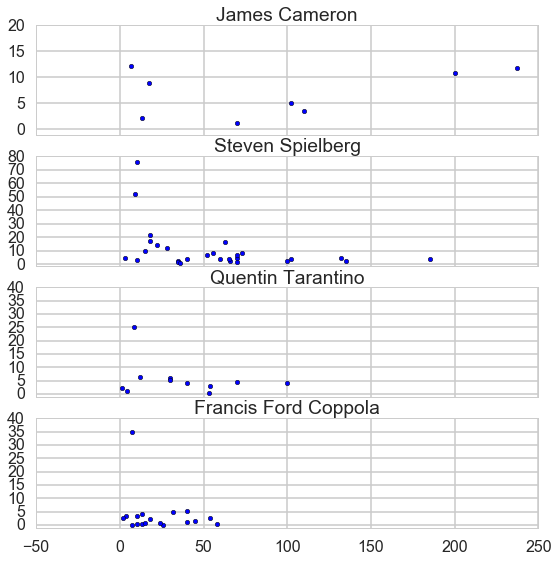
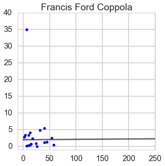
Movie investors always want to do best investment that can end up most return. The director is one of most significant factor to achieve this goal. Therefore it worth to predict profit given a certain amount of budget based on their historical records.
At this time, I only analyze four famous science fiction directors: James Cameron, Steven Spielberg, Quentin Tarantino and Francis Ford coppola.
Results
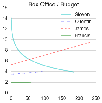
Ratio of box office and budget
From this ratio figure, if budget is less than $100 million Steven is the best; whereas if budget is larger than $100 million James is outstanding.
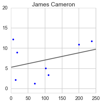
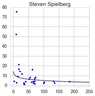
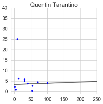
Ratio of box office and budget
From this ratio figure, if budget is less than $55 million Steven is the best; whereas if budget is larger than $55 million James is outstanding.
Takeaway points
Be careful with the outliers, rule them out before apply regression.
Find the right function to fit the data.
The ratio cannot be negative, so we need to consider this when we choose function to fit data. When I fitted the ratio for Steven, I applied logorithm function.
Further works
Scrape more directors and add some more features, like genre, producer and editor.
The ideal final product should be a we page that you can input features then it will output the rank list of directors.
Detailed process
Scrape data from wiki
James Cameron
#https://en.wikipedia.org/wiki/James_Cameron_filmographydirector='James_Cameron'url='https://en.wikipedia.org/wiki/'+director+'_filmography'#Apply this header to avoid being denied.headers={'user-Agent':'Mozilla/5.0'}response=requests.get(url,headers=headers)page=response.textsoup=BeautifulSoup(page,"lxml")tables=soup.find_all('table')#Check the tables visually and then get what we want.tables=tables[0]James_data=[]rows=tables.find_all('tr')forrowinrows[2:]:row_dict={}th=row.find('th')th_ref=th.find('a')ifth_refisnotNone:year=row.find('td')ifyear.findNextSibling().get_text()=='Yes':#Make sure he is the directorrow_dict['Title']=th_ref.get_text()row_dict['Year']=year.get_text()row_dict['url']=th_ref['href']James_data.append(row_dict)James_df=pd.DataFrame(James_data)James_df.head(2)
Title
Year
url
0
Xenogenesis
1978
/wiki/Xenogenesis_(film)
1
Piranha II: The Spawning
1981
/wiki/Piranha_II:_The_Spawning
Now we got the table which contains all movies that James direct and have a hyperlink so that we can find detailed information. Then I define a function to scrape budget and box office values based on this table.
Then we need to define another function to clean this table.
defclean_num(bucks):bucks=bucks.replace(',','')nums=re.findall('[0-9.]{2,}',bucks)#find the number who has more than 2 digitsiflen(nums)==0:nums=re.findall('[0-9.]+ [a-z]+',bucks)#find the number + character combinationiflen(nums)==0:returnNoneelse:nums=re.findall('\d',nums[0])mil=re.findall('million',bucks)bil=re.findall('billion',bucks)iflen(mil)>0:unit='million'eliflen(bil)>0:unit='billion'else:unit='digit'ifunit=='million':nums=[np.float(x)forxinnums]ifunit=='billion':nums=[np.float(x)*1000forxinnums]ifunit=='digit':nums=[np.float(x)/1000000forxinnums]res=np.mean(nums)returnresJames_df['Box office']=James_df['Box office'].apply(clean_num)James_df['Budget']=James_df['Budget'].apply(clean_num)James_df.head(2)
Title
Year
url
Box office
Budget
2
The Terminator
1984
/wiki/The_Terminator
78.300000
6.4
3
Aliens
1986
/wiki/Aliens_(film)
157.200000
17.5
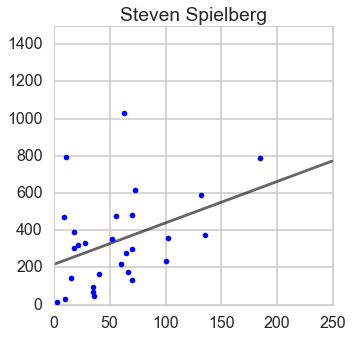
Steven Spielberg
#https://en.wikipedia.org/wiki/James_Cameron_filmographydirector='Steven_Spielberg'url='https://en.wikipedia.org/wiki/'+director+'_filmography'#Apply this header to avoid being denied.headers={'user-Agent':'Mozilla/5.0'}response=requests.get(url,headers=headers)page=response.textsoup=BeautifulSoup(page,"lxml")tables=soup.find_all('table')tables=tables[2]
For this table there are some years span over multiple movies, so we need to take care of this situation.
Steven_data=[]header=['Title','Year','url']rows=tables.find_all('tr')forrowinrows[1:]:row_dict={}td=row.find_all('td')td0=td[0].get_text()check_td0=re.findall('[0-9]{4,}',td0)#Find number that has more than 3 digitsifcheck_td0!=[]:year=td[0].get_text()if(td[1].aisnotNone)andtd[2].get_text()=='Yes':row_dict['Title']=td[1].get_text()row_dict['Year']=yearrow_dict['url']=td[1].a['href']Steven_data.append(row_dict)else:#The first cell is not year so it has spanned year.if(td[0].aisnotNone)andtd[1].get_text()=='Yes':row_dict['Title']=td[0].get_text()row_dict['Year']=yearrow_dict['url']=td[0].a['href']Steven_data.append(row_dict)Steven_df=pd.DataFrame(Steven_data)Steven_df.Year=pd.to_numeric(Steven_df.Year)Steven_df=Steven_df[Steven_df.Year<2016]#We only want movies that have already been screened.Steven_df.head(2)
Title
Year
url
0
Amblin’
1968
/wiki/Amblin%27
1
Duel
1971
/wiki/Duel_(1971_film)
Scrape box office and budget values. Merge and clean table.
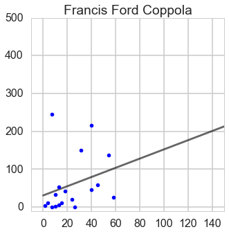
lm=LinearRegression()y_Francis=Francis_df['Box office']X_Francis=Francis_df['Budget']X_Francis=sm.add_constant(X_Francis)lm.fit(X_Francis,y_Francis)line_X=np.arange(0,250)line_X=sm.add_constant(line_X)line_X=pd.DataFrame(line_X)line_y=lm.predict(line_X)plt.plot(line_X.iloc[:,1],line_y,'-k',alpha=0.6)plt.plot(X_Francis.iloc[:,1],y_Francis,'.b')plt.title('Francis Ford Coppola')plt.xlim(-10,250)plt.ylim(-10,3000)fig=plt.gcf()fig.set_size_inches(8,8)plt.show()
This data set has 10 features diabetes.data and one target diabetes.target. Besides, there is no description of this data set, so we need to do some feature engineering first.
Feature Engineering
Remember that the first thing for feature engineering is to imagine you are the expert in that specific area that your data comes from. From expert perspective, you can select features based on professional experience (just google it as much as you can).
1. Check whether this data set is normalized
X=diabetes['data']X=DataFrame(X)X.describe()
We can tell from this description of each feature that the mean value is around 0 and has same standard deviation. Therefore, the predictors are normalized.
In other datasets, the X may not be centered, then we need to add the intercept. In sklearn, there is one argument to add intercept fit_intercept = True. The alternative way is:
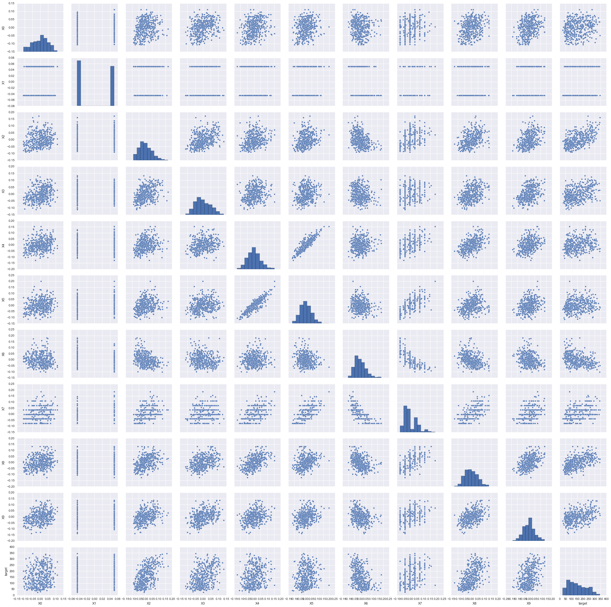
3. Plot the scatter points of each feature against target
From the pair plot figure we can tell the relationship of features and target and the relationship between features. There may be some features do not have linear relationship with target, we can try to guess any function in our knowledge have the similar curves with those nonlinear relationship. If we detect some strong correlated features, we should be really careful. When two features are linearly correlated, we need to remove one of them from analysis. When two features have nonlinear relationship, we still need to guess the function that can describe this relationship best.
sns.pairplot(diabetes_df)
We can tell from this pair plot figure that there are two categorical features and it is not necessary to apply polynomial regression.
Split the data
Since we need to compare the results from multiple models, we need to split the data into train and test sets.
In this case, we need to shuffle the data before we split data. However in some other cases, we need to apply different strategies. If the data is in time series, then we may not need to shuffle the data. If target is categorical, then we need to use stratified k-fold.
Cross Validation
Now we need to apply cross validation to choose tuning parameter in regularized models.
In this case, we need to shuffle the data before we split data (even if the data is in time series). If target is categorical, then we need to use stratified k-fold.
fromsklearn.cross_validationimportStratifiedKFoldX=np.array([[1,2],[3,4],[1,2],[3,4]])y=np.array([0,0,1,1])skf=StratifiedKFold(y,n_folds=2)fortrain_index,test_indexinskf:print("TRAIN:",train_index,"TEST:",test_index)X_train,X_test=X[train_index],X[test_index]y_train,y_test=y[train_index],y[test_index]#Then fit and test your model.
TRAIN: [1 3] TEST: [0 2]
TRAIN: [0 2] TEST: [1 3]
2. Select best tuning parameter
Apply grid search and cross validation to find the optimal tuning parameters in the lasso, ridge and elastic net models. Compared with lasso penalty, ridge (L2) penalizes less on small numbers and more on large numbers. Elastic net tries to balance these two penalties.
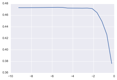
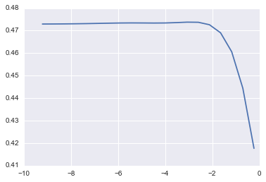
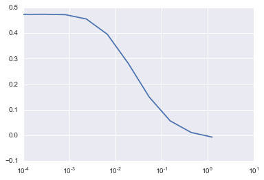
defcv_optimize(clf,parameters,X,y,n_folds,n_jobs=1,score_func=None):ifscore_func:gs=GridSearchCV(clf,param_grid=parameters,cv=n_folds,n_jobs=n_jobs,scoring=score_func)else:gs=GridSearchCV(clf,param_grid=parameters,n_jobs=n_jobs,cv=n_folds)gs.fit(X,y)print("BEST",gs.best_params_,gs.best_score_)df=pd.DataFrame(gs.grid_scores_)#Plot mean score vs. alphaforparaminparameters.keys():df[param]=df.parameters.apply(lambdaval:val[param])plt.semilogx(df.alpha,df.mean_validation_score)returngs
1) Lasso
params = {
    "alpha": np.logspace(-4, -.1, 20)
}
#If we do not know whether we need to normalize the data first, we can do this:
#params = {
#    "alpha": np.logspace(-4, -.1, 20), "normalize": [False, True]
#}
lm_lasso = cv_optimize(Lasso(), params, X_train, y_train, kfold)
Now we will fit the linear regression models with or without penalties.
lm_lasso_best=Lasso(alpha=lm_lasso.best_params_['alpha']).fit(X_train,y_train)lm_ridge_best=Lasso(alpha=lm_ridge.best_params_['alpha']).fit(X_train,y_train)lm_elasticnet_best=Lasso(alpha=lm_elasticnet.best_params_['alpha']).fit(X_train,y_train)lm_base=LinearRegression().fit(X_train,y_train)y_lasso=lm_lasso_best.predict(x_holdout)y_ridge=lm_ridge_best.predict(x_holdout)y_elasticnet=lm_elasticnet_best.predict(x_holdout)y_base=lm_base.predict(x_holdout)mse_lasso=np.mean((y_lasso-y_holdout)**2)mse_ridge=np.mean((y_ridge-y_holdout)**2)mse_elasticnet=np.mean((y_elasticnet-y_holdout)**2)mse_base=np.mean((y_base-y_holdout)**2)print("Linear Regression: R squred score is ",r2_score(y_holdout,y_base)," and mean squred error is ",mse_base)print("Lasso Regression: R squred score is ",r2_score(y_holdout,y_lasso)," and mean squred error is ",mse_lasso)print("Ridge Regression: R squred score is ",r2_score(y_holdout,y_ridge)," and mean squred error is ",mse_ridge)print("Elastic Net Regression: R squred score is ",r2_score(y_holdout,y_elasticnet)," and mean squred error is ",mse_elasticnet)
Then we can choose the best models with best R squred score and mean squared errors.
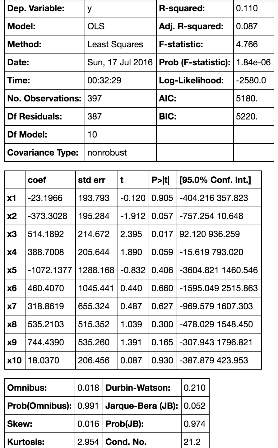
More statistics
In many situations, we want to check more statistics of linear regression. We can apply t statistic to select features with base linear regression. The smaller p-value of t statistic means more significance of that feature. Typically when p-value is larger than 0.05 we say that feature is not important. To do this, we need to use package statsmodels.api.
#X_train = sm.add_constant(X_train) #if data is not centered.model=sm.OLS(y_train,X_train)results=model.fit()results.summary()
This table can provide a lot of statistical analysis information. From this table, if we set significance level as 0.05 there are only two significant features. However we still cannot simply decide to get rid of those unimportant features.
Check specific features
If some features are ruled out by regularization regression or have very large p-value, we need to plot the points and fitted line to make a double check. It may be caused by noisy features, non-linear relationship or correlated features.
Xt=X_train[:,2]#Check third feature.X_line=np.linspace(min(Xt),max(Xt),10).reshape(10,1)X_line=np.tile(X_line,[1,10])y_train_pred=lin_reg_est.predict(X_line)plt.scatter(Xt,y_train,alpha=0.2)plt.plot(X_line,y_train_pred)plt.show()
Some further discussion about normalization (centering and scaling):
centering is equivalent to adding the intercept
when you’re trying to sum or average variables that are on different scales, perhaps to create a composite score of some kind. Without scaling, it may be the case that one variable has a larger impact on the sum due purely to its scale, which may be undesirable.
To simplify calculations and notation. For example, the sample covariance matrix of a matrix of values centered by their sample means is simply \(X′X\). Similarly, if a univariate random variable \(X\) has been mean centered, then \(var(X)=E(X^2)\) and the variance can be estimated from a sample by looking at the sample mean of the squares of the observed values.
PCA can only be interpreted as the singular value decomposition of a data matrix when the columns have first been centered by their means.
Note that scaling is not necessary in the last two bullet points I mentioned and centering may not be necessary in the second bullet I mentioned, so the two do not need to go hand and hand at all times. For regression without regularization centering and scaling are not necessary, but centering is helpful for interpretation of coefficients. For regularized regression, centering (or adding intercept) is necessary because we want coefficients have same magnitude.
Remarks and Tips
If the data size is very large, then grid search and cross validation will cost too much time. Therefore we may use small number of folds and small candidate sets of parameters.
Before split data and fit model you need to make sure that your features are in columns. Especially when you have only one feature, you may apply np.reshape().
If the data set was not centered, we need to set the intercept = True inside each model.
sklearn and statsmodels.api apply different algorithm to fit the linear model, so they will out put different results.
Another way to use regularization models is to apply them select features, then use base linear regression to analyze data with selected features
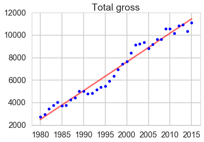
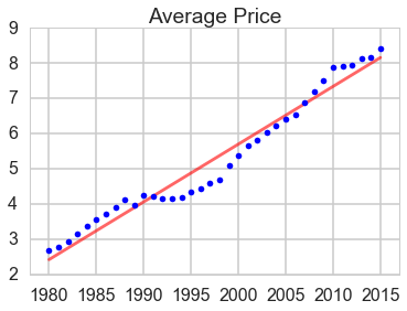
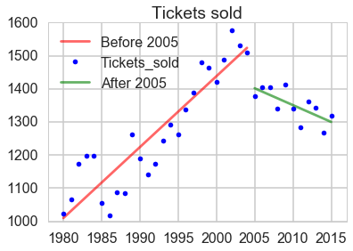
1. I will fit the yearly data with regression. The dataset is from Box Office Mojo. Specifically, the total gross, number of movies and average ticket price will be fitted against time with linear model and the number of tickets sold will be fitted with quadratic function. Based on fitted model we can predict the data in the future to help filmworkers to get a whole picture of future movie market.
2. I want to compare directors to see who can make more return on investment. To achieve this goal, I will use the regression model to get the relationship between budget and box office revenue for each director. This can provide some information to investors so that they will know to invest whom and what is the estimated profit. This is presented in the part 2
Results
Interesting findings
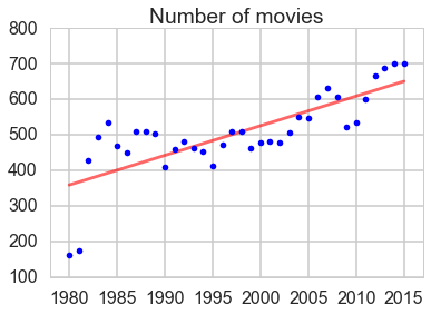
The total gross, number of movies and average price sold have an overall increasing trend.
The number of tickets sold had a big decline in 2005 and kept decreasing from then.
The average price of tickets increased faster from 2007.
The total gross fell in 2005 and the growth rate recovered in 2006.
Conjectures
The most likely reason for the decline of tickets sold is the rise of online movie providers. In 2005, YouTube was formed, in 2006 hulu is founded and in 2007 Netflix started to provide films online. So film workers should pay more attention on the international market.
Future works:
Study the international movie market trend. So that movie workers can find other faster developing morket to invest.
Analyze online movie service providers. Combine its result with what we got to see the whole movie market trend.
The detailed process is presented in the following.
Take-away points
When I scrape from some websites, some errors may be caused that web site do not have a perfect coding patern.
Unicode will pop up some times.
Presentation slides
Detailed Process
Prepreparation in python 3
1. Import some necessary packages
importpandasaspdfrompandasimportDataFrameimportnumpyasnpimportmatplotlib.pyplotaspltfrombs4importBeautifulSoupimportrequestsfromsklearn.linear_modelimportLinearRegressionimportseabornassnssns.set_style("whitegrid")sns.set_context("poster")importstatsmodels.apiassm# special matplotlib argument for improved plotsfrommatplotlibimportrcParamsimportre
url='http://www.boxofficemojo.com/yearly/'#Apply this header to avoid being denied.headers={'user-Agent':'Mozilla/5.0'}response=requests.get(url,headers=headers)#Check whether you request is successfulresponse.status_code
If status_code shows 200, it means the request is successful.
Then we need to check each table to see if there is some properties that can specify the table we want. Unfortunately, there is no such properties. So we need to visually check tables. After this step we know table[2] is what we want.
movie_data=[]movie_list=tables[2]#header can also be scraped. But some times we want to give a better header.header=['Year','Total_gross','Change1','Tickets_sold','Change1','num_movies','total_screens','Ave_price','Ave_cost','movie_1']rows=[rowforrowinmovie_list.find_all("tr")]forrowinrows[1:]:row_dict={}fori,cellinenumerate(row.findAll("td")):row_dict[header[i]]=cell.get_text()movie_data.append(row_dict)movies_df=pd.DataFrame(movie_data)# Get rid of the $ sign.
Then we need to clean this table: transform some string type to numeric and remove some special signs.
df1=movies_df.drop(0)#remove the data in 2016movies_df=movies_df.drop(0)# The first does not have whole year datamovies_df.to_csv('df_yearly.txt',index=False)
lm=LinearRegression()y2=df1.num_movieslm.fit(X1,y2)line_X=np.arange(df1.Year.min(),df1.Year.max()+1)line_X=sm.add_constant(line_X)line_y=lm.predict(line_X)plt.plot(line_X[:,1],line_y,'-r',label='Linear regressor',alpha=0.6)plt.plot(X1.iloc[:,1],y2,'.b',label='test')plt.title('Number of movies')plt.xlim(1978,2017)plt.legend(loc=2)plt.show()print(lm.score(X1,y2))