Problem Statement
1. I will fit the yearly data with regression. The dataset is from Box Office Mojo. Specifically, the total gross, number of movies and average ticket price will be fitted against time with linear model and the number of tickets sold will be fitted with quadratic function. Based on fitted model we can predict the data in the future to help filmworkers to get a whole picture of future movie market.
2. I want to compare directors to see who can make more return on investment. To achieve this goal, I will use the regression model to get the relationship between budget and box office revenue for each director. This can provide some information to investors so that they will know to invest whom and what is the estimated profit. This is presented in the part 2
Results
Interesting findings
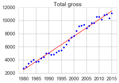
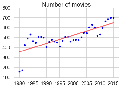
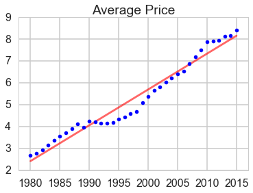
- The total gross, number of movies and average price sold have an overall increasing trend.
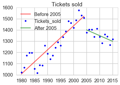
- The number of tickets sold had a big decline in 2005 and kept decreasing from then.
- The average price of tickets increased faster from 2007.
- The total gross fell in 2005 and the growth rate recovered in 2006.
Conjectures
The most likely reason for the decline of tickets sold is the rise of online movie providers. In 2005, YouTube was formed, in 2006 hulu is founded and in 2007 Netflix started to provide films online. So film workers should pay more attention on the international market.
Future works:
- Study the international movie market trend. So that movie workers can find other faster developing morket to invest.
- Analyze online movie service providers. Combine its result with what we got to see the whole movie market trend.
The detailed process is presented in the following.
Take-away points
- When I scrape from some websites, some errors may be caused that web site do not have a perfect coding patern.
- Unicode will pop up some times.
Presentation slides
Detailed Process
Prepreparation in python 3
1. Import some necessary packages
import pandas as pd
from pandas import DataFrame
import numpy as np
import matplotlib.pyplot as plt
from bs4 import BeautifulSoup
import requests
from sklearn.linear_model import LinearRegression
import seaborn as sns
sns.set_style("whitegrid")
sns.set_context("poster")
import statsmodels.api as sm
# special matplotlib argument for improved plots
from matplotlib import rcParams
import re
Yearly data analysis
Scraping data from Box Office Mojo
url = 'http://www.boxofficemojo.com/yearly/'
#Apply this header to avoid being denied.
headers = {
    'user-Agent': 'Mozilla/5.0'
}
response = requests.get(url, headers = headers)
#Check whether you request is successful
response.status_code
If status_code shows 200, it means the request is successful.
page = response.text
soup = BeautifulSoup(page)
tables = soup.find_all('table')
Then we need to check each table to see if there is some properties that can specify the table we want. Unfortunately, there is no such properties. So we need to visually check tables. After this step we know table[2] is what we want.
movie_data = []
movie_list = tables[2]
#header can also be scraped. But some times we want to give a better header.
header = ['Year','Total_gross','Change1', 'Tickets_sold', 'Change1', 'num_movies','total_screens',
         'Ave_price', 'Ave_cost', 'movie_1']
rows = [row for row in movie_list.find_all("tr")]
for row in rows[1:]:
    row_dict={}
    for i,cell in enumerate(row.findAll("td")):
        row_dict[header[i]] = cell.get_text()
    movie_data.append(row_dict)
movies_df = pd.DataFrame(movie_data)
# Get rid of the $ sign.
Then we need to clean this table: transform some string type to numeric and remove some special signs.
movies_df.Total_gross = movies_df.Total_gross.str[1:]
movies_df.Total_gross = movies_df.Total_gross.str.replace(',', '')
movies_df.Total_gross = pd.to_numeric(movies_df.Total_gross)
movies_df.Ave_price = movies_df.Ave_price.str.lstrip("$")
movies_df.Total_gross = pd.to_numeric(movies_df.Total_gross)
movies_df.Year = pd.to_numeric(movies_df.Year)
movies_df.Tickets_sold = movies_df.Tickets_sold.str.replace(',', '')
movies_df.Tickets_sold = pd.to_numeric(movies_df.Tickets_sold)
movies_df.num_movies = pd.to_numeric(movies_df.num_movies)
movies_df.head()
| Ave_cost | Ave_price | Change1 | Tickets_sold | Total_gross | Year | movie_1 | num_movies | total_screens | |
|---|---|---|---|---|---|---|---|---|---|
| 0 | - | 8.58 | - | 715.3 | 6137.0 | 2016 | Finding Dory | 362 | - |
| 1 | - | 8.43 | +4.1% | 1320.1 | 11128.5 | 2015 | Star Wars: The Force Awakens | 701 | - |
| 2 | - | 8.17 | -5.6% | 1268.2 | 10360.8 | 2014 | American Sniper | 702 | - |
| 3 | - | 8.13 | -1.3% | 1343.6 | 10923.6 | 2013 | Catching Fire | 688 | - |
| 4 | - | 7.96 | +6.1% | 1361.5 | 10837.4 | 2012 | The Avengers | 667 | - |
Remember to write this data into your local file.
df1 = movies_df.drop(0)     #remove the data in 2016
movies_df = movies_df.drop(0)   # The first does not have whole year data
movies_df.to_csv('df_yearly.txt', index = False)
Linear Regression to fit data
Total gross
lm = LinearRegression()
y1 = df1.Total_gross
X1 = df1.Year
X1 = sm.add_constant(X1)
lm.fit(X1, y1)
line_X = np.arange(df1.Year.min(), df1.Year.max() + 1)
line_X = sm.add_constant(line_X)
line_y = lm.predict(line_X)
plt.plot(line_X[:, 1], line_y, '-r', label = 'Linear regressor', alpha = 0.6)
plt.plot(X1.iloc[:, 1], y1, '.b', label = 'test')
plt.title('Total gross')
plt.xlim(1978, 2017)
plt.legend(loc = 2)
plt.show()
print(lm.score(X1, y1))
0.96855021574507782
Number of movies
lm = LinearRegression()
y2 = df1.num_movies
lm.fit(X1, y2)
line_X = np.arange(df1.Year.min(), df1.Year.max() + 1)
line_X = sm.add_constant(line_X)
line_y = lm.predict(line_X)
plt.plot(line_X[:, 1], line_y, '-r', label = 'Linear regressor', alpha = 0.6)
plt.plot(X1.iloc[:, 1], y2, '.b', label = 'test')
plt.title('Number of movies')
plt.xlim(1978, 2017)
plt.legend(loc = 2)
plt.show()
print(lm.score(X1, y2))
0.58986278863620789
Average price
lm = LinearRegression()
y3 = df1.Ave_price
lm.fit(X1, y3)
line_X = np.arange(df1.Year.min(), df1.Year.max() + 1)
line_X = sm.add_constant(line_X)
line_y = lm.predict(line_X)
plt.plot(line_X[:, 1], line_y, '-r', label = 'Linear regressor', alpha = 0.6)
plt.plot(X1.iloc[:, 1], y3, '.b', label = 'data')
plt.title('Average Price')
plt.xlim(1978, 2017)
plt.legend(loc = 2)
plt.show()
print(lm.score(X1, y3))
0.96172045677804519
Number of tickets that were sold out
lm1 = LinearRegression()
lm2 = LinearRegression()
y4 = df1.Tickets_sold
X2 = X1
X2_2004 = X2[X2.Year <= 2004]
y4_2004 = y4[X2.Year <= 2004]
X2_2005 = X2[X2.Year > 2004]
y4_2005 = y4[X2.Year > 2004]
lm1.fit(X2_2004, y4_2004)
lm2.fit(X2_2005, y4_2005)
line_X1 = np.arange(X2_2004.Year.min(), X2_2004.Year.max() + 1)
line_X1 = sm.add_constant(line_X1)
line_X1 = pd.DataFrame(line_X1)
line_y1 = lm1.predict(line_X1)
line_X2 = np.arange(X2_2005.Year.min(), X2_2005.Year.max() + 1)
line_X2 = sm.add_constant(line_X2)
line_X2 = pd.DataFrame(line_X2)
line_y2 = lm2.predict(line_X2)
plt.plot(line_X1.iloc[:, 1], line_y1, '-r', label = 'Before 2005', alpha = 0.6)
plt.plot(X1.iloc[:, 1], y4, '.b', label = 'data')
plt.plot(line_X2.iloc[:, 1], line_y2, '-g', label = 'After 2005', alpha = 0.6)
plt.title('Tickets sold')
plt.xlim(1978, 2017)
plt.legend(loc = 2)
plt.show()
print((lm1.score(X2_2004, y4_2004) + lm2.score(X2_2005, y4_2005))/2)
0.655714846952